Construction
The three lines come from the same input series, the close:
- Middle band = SMA(close, 20)
- Upper band = SMA(close, 20) + 2 × stdev(close, 20)
- Lower band = SMA(close, 20) − 2 × stdev(close, 20)
Default parameters are (20, 2). At 2σ, a Gaussian distribution places about 95.4% of observations inside the envelope. Equity daily returns have kurtosis above 3, so the realised inside-band frequency typically sits between 88% and 93% rather than 95%. The discrepancy matters operationally. Any decision rule premised on “outside the band” being a 1-in-20 event is mis-calibrated by roughly a factor of two on liquid US names. Expect 1-in-30 days to break the linear projection in either direction.
The envelope is adaptive by construction. When realised volatility contracts, the stdev term shrinks and the bands pinch. When realised volatility expands, the stdev term grows and the bands widen. That is a feature, not a forecast. The bands describe what σ has been over the last 20 sessions. They say nothing about what σ will be over the next 20.
The Squeeze
The most-quoted Bollinger signal is the squeeze: a session where bandwidth, defined as (upper − lower) / middle, is at a multi-month low. A common operational threshold is current bandwidth in the bottom decile of the trailing 126 sessions, roughly six months of trading.
The empirical claim attached to the squeeze is that low realised volatility tends to be followed by higher realised volatility. Volatility clusters, and contraction precedes expansion. This is one of the more robust stylised facts in equity return data; the ARCH and GARCH families of models are built on exactly this property. Assuming the persistence parameter is approximately stationary across the lookback window, the squeeze-then-expansion pattern has positive expectancy on direction-neutral structures.
What the squeeze does not contain is direction. Bandwidth is a positive scalar. It has no sign. A low-bandwidth print is consistent with the next leg being a breakout either way. Strategies that take a directional read off the squeeze alone are inserting a prior the indicator does not carry. The methodologically clean approach is to wait for a close outside the envelope, then trade in that direction.
The Type-Signature Problem
This is where the programming analogy is useful. A bandwidth reading has a type signature: it is a non-negative real, returning a magnitude. It does not return a vector. Treating its output as if it carried direction is the trading equivalent of dereferencing a null pointer. The function does not return what you are asking it to return. The compiler — in this case, the P&L — will tell you eventually. It tends to tell you at size.
The fix is the same fix you apply when an API does not give you what you need: compose. Squeeze flags the regime; a directional indicator (close outside the envelope, momentum confirmation, volume on the breakout bar) supplies the sign. Two functions, two outputs, one decision. That composition is the signal template, not the squeeze itself.
Quantifying the Squeeze
A defensible rule: flag a squeeze when current bandwidth is in the bottom decile of the trailing 126 sessions. Entry is a close outside the envelope on volume at or above the 20-day average. Stop is the opposite band, or the middle band for a tighter version. Modulo transaction costs and the assumption that the bandwidth distribution is approximately stationary across the lookback, this framework has been tested broadly in the technical-analysis literature. The standard finding is small positive expectancy on liquid US large-caps, and approximately zero or negative expectancy on illiquid names once half-spread plus impact are modelled honestly.
Band Touches Are Not Signals
The second common error, after trading the squeeze directionally, is treating a band touch as an automatic reversal. It is not. In a trending regime, price walks the band — closing near or above the upper band for many consecutive sessions during an uptrend, with mirror-symmetric behaviour during a downtrend. Fading those touches is a negative-expectancy trade absent a regime filter.
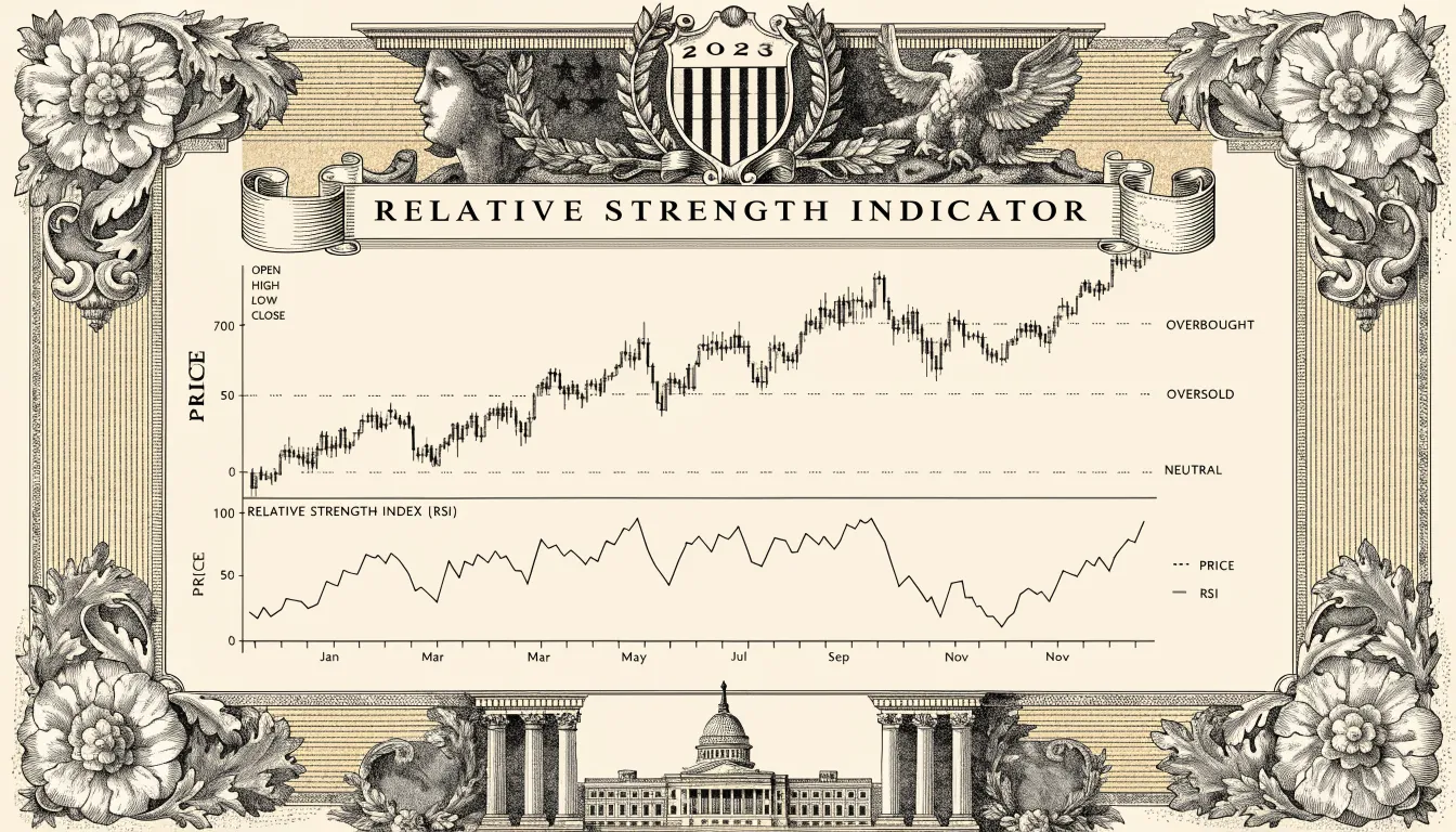
The conditional framing is more useful. A touch of the upper band combined with RSI above 70 on the same bar is a joint condition: price is statistically extended and momentum is overextended. Conversely, a touch of the lower band combined with RSI below 30 is a joint oversold condition. Bollinger Bands measure position within a recent volatility envelope; RSI measures momentum on a separate lookback. They are partially independent. Requiring both to agree reduces the false-signal rate without eliminating it.
A categorical clarification, which traders sometimes get wrong: the upper band is not a ceiling. It is a 2σ line computed off the last 20 closes. If a symmetrical triangle resolves on expanding volume, the resulting move pushes realised σ up, which widens the envelope on the next bar. The band moves with the price. It does not resist it. Treating a statistical envelope as a structural level is a category error of the same family as treating a moving average as support.
Settings and Variations
The default (20, 2) parameters are reasonable for liquid US equities on daily bars. Other combinations serve different timeframes and volatility regimes.
| Timeframe | Period | Std Dev | Use Case |
|---|---|---|---|
| Intraday | 10 | 1.5 | Faster response on 5–15 minute bars |
| Swing | 20 | 2.0 | Default on daily bars |
| Position | 20 | 2.0 | Weekly bars, longer horizons |
| High-volatility | 20 | 2.5 | Small caps, wide-gap names |
Widening to 2.5σ on small caps deserves explicit thought. On a name with high idiosyncratic volatility and frequent overnight gaps, the 2σ envelope is pierced often enough that the signal-to-noise ratio on band touches collapses toward zero. Widening to 2.5σ captures roughly 98.8% of a Gaussian distribution, and somewhat less in practice given the fat tails. The outside-band event becomes rarer and, conditionally, more informative. The cost is a later entry on genuine breakouts.
The parameter choice is a bias-variance tradeoff. Narrower bands and shorter periods produce more signals at a lower per-signal hit rate. Wider bands and longer periods produce fewer signals at a higher per-signal hit rate. There is no optimal setting independent of the name and the regime. Calibrate per universe, not per chart.
Common Failure Modes
Three recurring misuses of this indicator, in order of frequency.
Directional reads of the squeeze. As discussed, bandwidth has no sign. The clean response to a squeeze is to set conditional brackets above the upper band and below the lower band and let the market choose. Choosing for it is overriding the indicator with an outside prior, which may or may not be calibrated.
Fading band touches in a trending regime. Walking-the-band is a real phenomenon, well-documented on momentum names during sustained trends, and it will steadily decapitalise a mean-reversion trader who is not conditioning on trend. A simple filter — trade band touches only when the slope of the middle band is approximately flat within some tolerance, or when the ADX reading is below a regime threshold — removes most of the damage.
Using Bollinger Bands in isolation. They measure exactly one thing: position within a recent volatility envelope. They do not measure momentum, volume, breadth, or regime. MACD, RSI, and volume are complementary inputs, not redundant ones. Bollinger himself has been explicit that the indicator is a starting point, and that framing is accurate.
A Practical Workflow
A defensible Bollinger-based workflow for daily-bar swing trading on liquid names:
- Scan the universe for bandwidth in the bottom decile of the last 126 sessions.
- Set bracket orders one tick above the upper band and one tick below the lower band. Cancel at end of session if not filled.
- On a fill, require same-day volume at or above the 20-day average, and RSI moving in the direction of the breakout.
- Initial stop at the opposite band on close, or at the middle band for a tighter version.
- Trail the stop at the middle band. A close on the wrong side of the middle band closes the position.
This is a signal template, not a complete strategy. It carries no position-sizing rule, no portfolio-level risk budget, no treatment of earnings-day exposure, no transaction-cost model. Pulled out of those layers, it does not have a P&L. It has a hit rate and an expected payoff per trade, conditional on the layers being filled in elsewhere. Treat it as a function, not a service.
Closing Notes on Assumptions
Model assumptions, to be explicit. Bollinger Bands sit on an implicit Gaussian framing: 2σ is a meaningful boundary only if the underlying return distribution is approximately normal and approximately stationary. Equity returns are neither. They have kurtosis well above 3, skew that varies with the regime, and occasional regime shifts that break stationarity outright. Every number in this article — the 95% inside-band rate, the bottom-decile bandwidth threshold, the 2σ default, the 1-in-20 base rate — carries those assumptions with it.
That does not make the indicator useless. It makes it a specific tool with specific failure modes. The 2008 and 2020 regimes both produced extended periods where SPY daily returns had tails thick enough that 2σ touches happened on consecutive sessions — statistically near-impossible under a stationary Gaussian, perfectly normal under the actual data-generating process. A trader who insists on the Gaussian frame during those regimes will read every outside-band close as a reversal, and will be systematically wrong for as long as the regime persists.
Use Bollinger Bands as a volatility envelope with stated assumptions. Compose with a momentum filter and a volume filter. Condition on regime. Model transaction costs honestly. The indicator is a useful component. It is not a system, and treating it as one for any extended period has reliably produced losses.
See also: RSI: The Relative Strength Index · MACD: Moving Average Convergence Divergence · Moving Averages Explained · Understanding Volume · Support and Resistance · Technical Analysis · Triangle Patterns in Stock Trading